Introduction

Hello everyone, welcome back! today, I wanted to talk about the importance of efficiency with data structure and algorithms and how to use Big-O notation to measure the Time and Space complexity of an algorithm.

Efficiency

In my last post, we talked about how to solve computational problems with python but we didn't dive into whether our solution was efficient or not. That's what we will be looking at in this section.

Space and Time

When we refer to the efficiency of a program, we don't only look at the time it takes to run, but at the space required in the computer's memory as well. Often, there will be a trade-off between the two, where you can design a program that runs faster by selecting a data structure that takes up more space—or vice versa.

In order to quantify the time and space an algorithm takes, let's first understand what an algorithm is.

Algorithm

An algorithm is a series of well-defined steps for solving a problem. Usually, an algorithm takes some kind of input (such as a list) and then produces the desired output (such as a reversed list).

For any problem, there is likely more than one algorithm that can solve the problem, but there are some algorithms that are more efficient than others. However, computers are so fast! that in some problems, we can't tell the difference, so how can we know what algorithm is more efficient than another? and if we can't tell the difference, why try to make our code efficient?

Well, those are some great questions, and in some cases it's true, one version of a program may take 5 times longer than another, but they both still run so quickly that it has no real impact. However, in other cases, a very small change can make the difference between a program that takes milliseconds to run and a program that takes hours!.

Quantifying efficiency

Sometimes, you will hear programmers say:

"This algorithm is better than that algorithm"

But how can we be more specific than that? How do we quantify efficiency?.

Let's take a look at some code examples.

def add200(n):
    for i in range(2):
        n += 100
    return n

def add200_2(n):
    for i in range(100):
        n += 2
    return n

Both of the functions above have no real-world use, they are just dummy functions that will help us understand efficiency. Both of them add 200 to whatever the input(n) is. Take a good look at them and tell me, which one is more efficient?

The answer is the add200 function. Why?

Although both functions output the exact same result, the add200_2 function makes too many iterations, while the add200() function only iterates twice.

Counting Lines

With the example above, what we basically did was to estimate which code had more lines to run, let's take a look again at both functions

def add200(n):
    for i in range(2):
        n += 100
    return n

def add200_2(n):
    for i in range(100):
        n += 2
    return n

The first function has a total of 4 lines but because of the for loop that gets called twice, there is a total of 5 lines (the for loop line doesn't get counted).

Now, let's take a look at the second function. the total of lines is 4 but the for loop gets called 100 times! so running this code will involve running 103 lines of code!.

Counting lines it's not a perfect way of quantifying the efficiency of a program but it's an easy way for us to approximate the difference in efficiency between two solutions.

Input Size and How it Affects Efficiency

In both examples above, no matter what number we passed as an argument, the number of lines executed will remain the same.

Here's a new code example:

def print_to_num(n):
    for i in range(n+1):  # +1 because python counts from 0
        print(i)

print_to_num(10)

The code above prints all numbers from 0 to N, meaning the bigger the input N is, the number of lines executed will increase, and that means a longer time to run.

The highlighted idea it's that:

As the input to an algorithm increases, the time required to run the algorithm may also increase.

This may happen in some cases, in the last example it does increase the time, but in the first two, it does not.

Rate of increase

Let's keep working with the last function and let's try several function calls examples to see the number of lines each one gets to run.

print_to_num(2) # 4 lines
print_to_num(3) # 5 lines
print_to_num(4) # 6 lines
print_to_num(5) # 7 lines

As you can see, when N goes up by 1 the number of lines will also go up by 1. We can also say that the number of lines executed increases by a proportional amount. This type of relationship is called a Linear relationship if we graph the relationship we can see why it's called that.

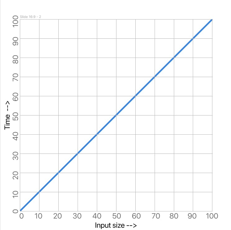
The x-axis represents the input size, in this case, a number, and the y-axis represents the number of operations that will be performed in this case we're thinking of an "operation" as a line of Python code which is not the most accurate but will do for now.

Let's take a look at another function example where the operations increase at a none constant rate.

def print_square(n):
    for i in range(1, n+1):
        for j in range(1, n+1):
            print("*", end="  ") # end=" " for printing all "*" in a single line separated by two white spaces
        print("") # this is used to mimic an "enter"

print_square(5)

This code prints a square made out of "*" that it's exactly N x N in size

output: 
*  *  *  *  *
*  *  *  *  *
*  *  *  *  *
*  *  *  *  *
*  *  *  *  *

Notice that this function has a nested loop, that means, a loop inside a loop, and take a good look at the fact that both loops have a linear rate of increase but they are nested that makes the rate of increase quadratic that means that when the input goes up by a certain amount, the number of operations goes up by the square of that amount.

print_square(1) # 1 line
print_square(2) # 4 lines
print_square(3) # 9 lines

Let's add the quadratic rate of increase to our graph:

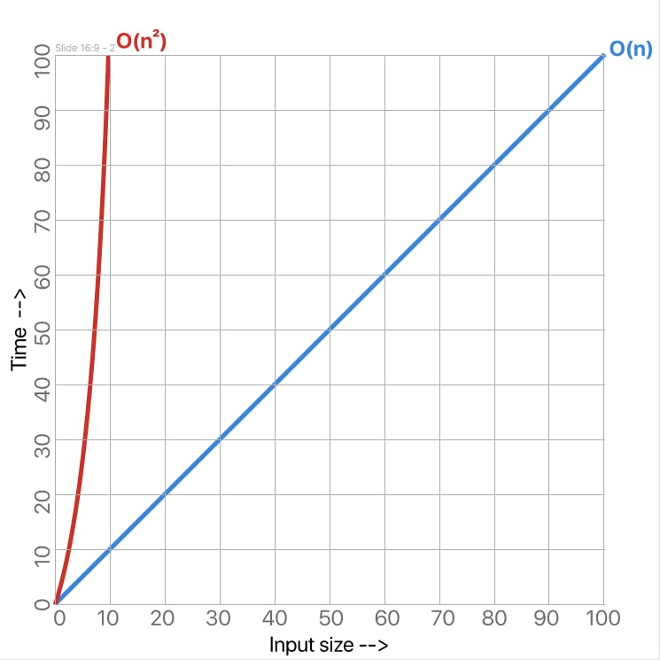
Our print_square function exhibits a quadratic rate of increase which as you can see is a much faster rate of increase, this means that as we pass larger numbers, the number of operations the computer has to perform shoots up very quickly making the program far less efficient These are only two examples of the rate of increase but there are many more. Here are the most common:

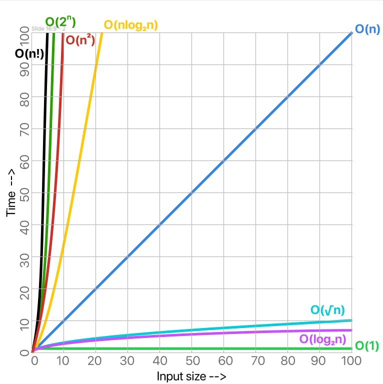
Note. when people refer to the rate of increase, they will often use the term "order". For example, instead of saying: "This algorithm has a linear rate of increase" they will say: "The order of this algorithm is linear"

Big-O notation

What is it?

Big-O notation is a "simplified analysis of an algorithm's efficiency". Big-O gives us an algorithm's complexity in terms of the input size (N) and it's independent of the machine we run the algorithms on. Big-O can give us the time but also space complexity of an algorithm

Types of Measurement

There are three types of ways we can look at an algorithm's efficiency.

1. Worst-case
2. Best-case
3. Average-case

Normally, when talking about Big-O notation we will typically look at the worst-case scenario, this doesn't mean the others are not used, but normally we want to know what the worst case is.

General Rules of Big-O

1. Big-O notation ignores constants. Example: let's say you have a function that has a running time of O(5n), in this case, we say that it runs on the order of O(n) because as N gets larger, the 5 no longer matters.

2. Terms priority. This means that if a function has a part that has an O(1) order but another part of that same function has an order of O(n) we will say that the whole function has an order of O(n). This includes sections that might not run, for example, in an if-else statement.

O(1) < O(logn) < O(n) < O(nlogn) < O(n2) < O(2n) < O(n!) (see graph above)

Code Examples

In this section, we will take a look at example lines of code and see how O(n) is used.

Constant Time O(1)

Take a look at the line below

print((5*10)/2) # outputs 25

As you can see, this code simply computes a simple math operation and it's not dependent on any input. This is an example of O(1) order or constant time.

What if we have not one but three simple math operations.

n = 5 + 2 # O(1)
y = 3 * 5 # O(1)
x = n + y # O(1)

Well, in this case, each line of code has an O(1) order, so what we need to do is add all of them like this: O(1)+O(1)+O(1) BUT let's remember the first rule and ignore constants, making the final result be O(1)

Linear Time O(n)

Let's try another example:

for i in range(n): # n * O(1) = O(n)
    print(i) # O(1)

The clearest example of Linear time code, it's a simple for loop that iterates from 0 to N. In the code shown above, the print statement has an order of O(1) but because it's inside a loop, we need to multiply O(1) * N which would give us a result of O(N)

If, for example, we had both examples above together like this:

n = 5 + 2 # O(1)
y = 3 * 5 # O(1)
x = n + y # O(1)
for i in range(n): # n * O(1) = O(n)
    print(i) # O(1)

We would have the O(1) of the simple math and print lines, and O(n) of the for loop, so, to calculate the total time we need to add both of them BUT let's remember our second rule of terms priority and make O(N) the final result for this code

Quadratic Time O(n²)

The easiest way to get a code to have a Quadratic order it's to simply have a nested loop with both of them iterating from 0 to N. Let's see the code example that we saw earlier:

def print_square(n):
    for i in range(1, n+1):
        for j in range(1, n+1):
            print("*", end="  ") # end=" " for printing all "*" in a single line separated by two white spaces
        print("") # this is used to mimic an "enter"

print_square(5)

The first for loop has a time complexity of O(N), the second for loop also has a time complexity of O(N), and finally, the print statements have a complexity of O(1). And hopefully, you can see pretty clearly that the print statement will be executed N * N times, making this whole code have a time complexity of O(N²)

If, we put all previous codes together like this:

n = 5 + 2 # O(1)
y = 3 * 5 # O(1)
x = n + y # O(1)

for i in range(n): # n * O(1) = O(n)
    print(i) # O(1)

for i in range(1, n+1): # O(n) * O(n) = O(n²)
    for j in range(1, n+1):
        print("*", end="  ")
    print("") # this is used to mimic an "enter"

we know the first code has a complexity of O(1) the second code has a complexity of O(n) and the third code has a complexity of O(n²) and because of our second rule, the complexity of the whole code it's O(n²)

Logarithmic Time O(log n)

An algorithm with a Logarithmic run time, it's that code that reduces the size of the input data in each step (it doesn't need to look at all values of the input data), a great example of this, is a Binary Search. Binary Search is a searching algorithm for finding an element's position in a sorted array.

def binary_search(arr, element):
    left = 0
    right = len(arr)-1
    while(left <= right):
        mid = (left + right)//2
        if arr[mid] == element:
            return mid
        if arr[mid] < element:
            left = mid +1
        else:
            right = mid -1
    return -1

print(binary_search([1,2,3,4,5,6,7,8,9], 8))

Log-Linear Time (O(n log n))

An algorithm is said to have a log-linear time complexity when each operation in the input data has a logarithm time complexity. It is commonly seen in sorting algorithms

codes = set()
for phone in phones_arr:
    codes.add(phone[:4])
print('\n'.join(sorted(codes))) # <== O(n log n)

The code above iterates through an array of phone numbers and adds the first four digits of each phone to a "codes" set(a set doesn't allow duplicates) and finally the code prints the codes but are sorted.

Exponential Time O(2ⁿ)

Algorithms have an exponential time complexity when the growth doubles with each addition to the input data set. This kind of time complexity is usually seen in brute-force algorithms.

def fibonacci(n):
    if n <= 1:
        return n
    return fibonacci(n-1) + fibonacci(n-2)

print(fibonacci(8)) # outputs 21

A great example of an exponential time algorithm is the recursive calculation of Fibonacci numbers, the code above receives a number and prints the N number in the Fibonacci sequence: 0, 1, 1, 2, 3, 5, 8, 13, 21

Factorial Time

An algorithm where the operational execution complexity increases factorially with the increase in the input size. As you can see from the graph above, this is the most inefficient order that an algorithm can have.

def factorial(n):
    if n == 1:
        return n
    else:
        return n * factorial(n-1)

print(factorial(4))

The function above receives a number and uses recursion to print the result of multiplying all numbers from 1 to N 4*3*2*1 = 24

Conclusion - Farewell

You've reached the end of this post on complexity and Big-O notation to quantify time efficiency, I really hope some of the concepts we saw today have helped you and hopefully you will be thinking not only about solving a problem but to think weather your code is efficient or not. If you liked this post, make sure to share it with another person that might find this interesting, and let me know in the comments your thoughts, suggestions, and what you will like to see next.

See you in the next post, stay tuned for more!