Introduction

Hey there, fellow coders! Today, we're going to navigate through the exciting world of dynamic programming, tackling a captivating competitive programming problem along the way. We'll be stepping into the shoes of game strategists, playing a turn-based game over an array where every decision counts.

Imagine this: you're playing a game where you and your opponent take turns removing elements from either end of an array. The challenge? Both of you are top-notch strategists aiming to maximize your own sums. Sounds intriguing, right?

So, let's roll up our sleeves, dive deep into the strategy of optimal play, and discover how we can wield the power of dynamic programming to solve this challenge. Ready to unlock a new level of your programming skills? Let's get started!

"Optimal Play" Problem

There is a very popular game that's creating quite a buzz. This two-player game revolves around a linearly arranged set of N coins, each represented by a number indicating its value. The crux of the game? To amass the maximum possible wealth. On each turn, a player can choose to take either the coin at the beginning or the end of the line. This back-and-forth continues until the last coin has been claimed.

In a bold move, you've invited your math teacher - a formidable opponent known for his strategic prowess - to a round of this game. Confident in his abilities, he's even let you take the first turn. Your mission, should you choose to accept, is to devise a program that, given an array of coins, predicts the maximum wealth you can amass. The catch? Both you and your teacher are playing optimally.

Inputs:

Your program will be receiving two lines of input:

1. The first line will contain a single integer N, where 1 <= N <= 1000. This number represents the size of the line of coins.

2. The second line will contain N space-separated integers. Each of these integers represents the value of a coin in the line and will be between 1 and 1,000,000,000 (1E9), inclusive.

Outputs:

Your program should output a single line containing one integer, representing the maximum amount of money you can win by playing this game optimally. Remember, you're making the first move and both you and your opponent are expected to play in the most strategic manner.

Example:

Now that we have understood the problem, let's see an example to bring our understanding to life.

Input:

5
1 3 5 2 9

Output:

15

Explanation:

In this game, we start with a line of 5 coins with the values 1, 3, 5, 2, and 9, in that order. We take the first turn, and both we and our opponent play optimally.

• First, we take the coin with the value 9 (since it's the highest value), leaving the line as 1, 3, 5, 2.

• Our opponent, playing optimally, would take 2 (leaving 1, 3, 5 as our options).

• On our turn, we take the coin with value 5, leaving the line as 1, 3.

• Our opponent now takes the coin with value 3, leaving only 1 in the line.

• Finally, we take the last coin, which is 1.

So, in total, we have taken coins of values 9, 5, and 1, summing up to 15, which is the maximum amount of money we can win in this scenario. Hence, the output is 15.

Greedy Approach

Upon the first encounter, this problem might seem like a cakewalk. The seemingly straightforward approach would be to opt for the largest available value at each turn and repeat the same strategy for our opponent. Essentially, we're simulating the entire game by iterating through the array in a specific order. With the time and space complexity of O(N), this approach is undoubtedly efficient.

The viability of this strategy shines through in our initial example and even holds up when tested on an example such as:

4
1 2 3 4

However, as the good competitive programmers that we are, we should question more if this solution is correct by trying to create an example in which this solution does not work.

4
20 30 2 2

If we follow the greedy approach:

• We first pick 20, leaving the line as 30, 2, 2.

• Then our opponent picks 30, leaving the line as 2, 2.

• We pick 2, leaving the line as 2.

• Lastly, our opponent picks the final 2.

Here, we've ended up with coins worth 20 + 2 = 22.

However, if we played optimally, considering our opponent also plays optimally:

• We first pick 2 from the end, leaving the line as 20, 30, 2.

• Our opponent, playing optimally, picks 20, leaving the line as 30, 2.

• We pick 30, leaving the line as 2.

• Lastly, our opponent picks the final 2.

So, playing optimally, we would end up with coins worth 2 + 30 = 32, which is the correct and maximum achievable sum considering both players are playing optimally.

This example clearly demonstrates that the greedy approach doesn't always result in the best outcome, emphasizing the importance of a strategy that considers future moves and the optimal plays of the opponent.

Brute Force Approach

It might be tempting to dissect the shortcomings of our initial greedy strategy until we're utterly convinced of its flaws. But really, that single example where it fell short is quite enough to nudge us away from it, encouraging us to think creatively and explore other strategies.

One such strategy that often comes to mind during these times is the Brute Force approach. If you're new to this concept, it's actually quite simple. All it means is that we try out every possible game scenario. Although this usually gives us the right answer, it can be a bit slow. But no worries - for now, our main aim is to find a solution that works, no matter how slow. We can always speed things up later to avoid hitting any time limits.

Remember, problem-solving isn't always about finding the quickest solution, but about finding a solution that works. Then, we can always improve and refine it!

Implementation

Picture a maze where you're standing at the entrance, looking to navigate through different routes to find the exit. That's kind of like what we're trying to do here - explore all possible 'paths' of the game, using what's called a recursive approach.

Imagine each decision we make as branching off into a tree-like structure of different outcomes (See the image).

Notice how quickly our 'decision tree' expands. But no worries, we'll tackle this size issue later.

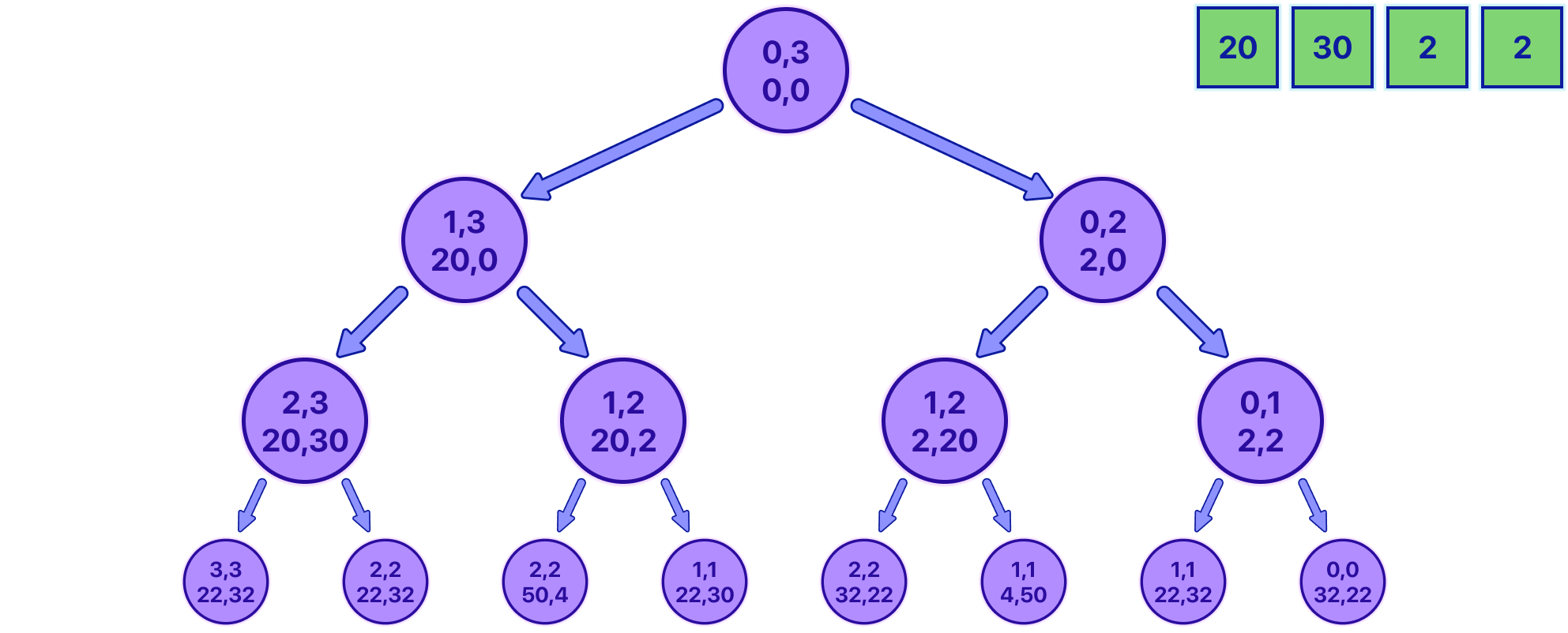
Let's break down this decision tree, starting from the first node. Each node represents a snapshot of our game, defined as: {LeftIndex, RightIndex, Sum1, Sum2}. Here, 'Sum1' and 'Sum2' are the total values of coins you and your opponent have respectively, starting at 0. The 'LeftIndex' and 'RightIndex' mark the inclusive range of coins left to play with. At the start of the game, this range covers the whole array, hence why it starts at 0 and ends at 3.

Each node offers two decisions:

• Grab the coin from the left of the array, which means adding the value of the coin at 'LeftIndex' to your total (or your opponent's, depending on whose turn it is), and then moving the 'LeftIndex' one step to the right (essentially 'removing' that coin from the game).

• Grab the coin from the right, which means adding the coin at 'RightIndex' to the current player's total, and then moving the 'RightIndex' one step to the left.

Notice that when both indices are equal there is no need to create a new node, and we can directly add the value at the index to however the player was supposed to play on the next move.

Hopefully, by knowing this you can better see how the Tree represents all possible ways a game can unfold.

Initially, I thought of simply finding the path that maximized your sum, however, by looking at the tree, I realized that if I do that, the code is going to output 50, which is an incorrect output because of the fact that we are not considering that the opponent is guaranteed to play in the most optimal way possible.

This adds another layer of complexity, but no worries, it's manageable.

A key question here is: "Can we predict the opponent's best move from any given node?" If we could, we'd simply choose the opposite option, aiming to minimize the opponent's total. Let's visualize it to get a better understanding:

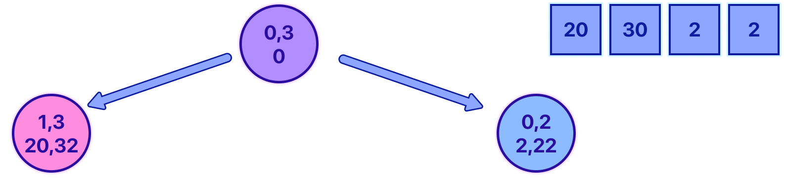
Imagine you're at the purple node, deciding whether to go left or right. If we knew that the best move for the opponent would lead us to the pink node, we'd instead move to the blue node - after all, when your opponent isn't doing well, you are.

Unfortunately for us, there is no way for us to know the optimal play for the opponent until we have explored the full path. realizing that the only way for us to know the optimal value is by going down the tree is key because it allows us to change our perspective. Instead of trying to solve the problem from the root, we are going to start from the leaves.

Starting from the leaves makes a ton of sense because it's the only point in time when we know the best decision with certainty.

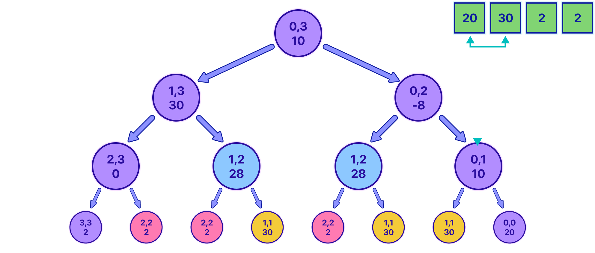
In the animation above, notice how the pink nodes represent states in which is your turn, and the purple nodes represent states for the opponent. At the beginning, we start at the root node and explore to the right and then to the left for each node, we continue exploring until we reach a base case that marks when a leaf is met. The base case is very simple, it's just when the indexes are equal.

Observe how in the animation, it can be shown up until the point in which you have the information to fill the first two leaves 1,1 and 0,0, and now the parent 0,1 state must be filled.

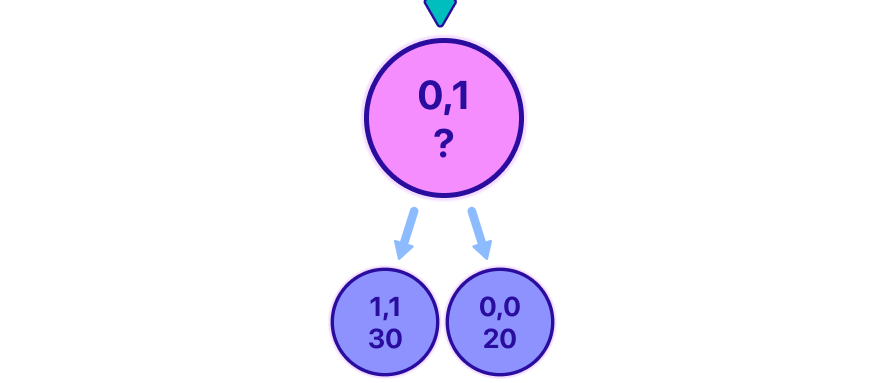
We're trying to figure out what value the pink node should have. At first, we might want to generalize and think that the value for all nodes should represent the highest possible score we can get from that range of coins.

But when we look at the values of the two nodes beneath the pink node (its children), we only really know which option is better for us. In this situation, if we take a step to the left, the other player (the opponent) will have a chance to earn more than if we take a step to the right. So, we want to choose the option that is worse for the opponent. However, knowing this doesn't tell us what our total score will be for that range of coins. We need to think a bit harder about this problem and consider it from different angles.

What we can do for the value of each node is, instead of saving the maximum earning possible from a range, we save the maximum advantage possible. Let's look more into this idea.

Notice how the leaves stay the same since it's still the correct value with this new logic. But now let's try to fill the value for the pink node.

val = max(-leftChild + arr[l], -rightChild + arr[r])

Let's break down the line above with the help of the image below.

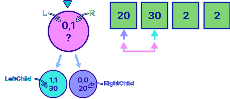
The left child contains the maximum advantage it can be obtained from the range [1,1], which in this case, it's 30, trivial because it's the case in which the indexes are the same. For the right child, it's the same leaf case, now with a value of 20. Now, for the pink node, we know for sure that both of the children are going to represent the maximum advantage but for the opponent, this is important, because it means that it's not going to be your advantage. This is the reason we make both children nodes negative when calculating the pink value, and of course, we must not forget to sum the value that made the left and right states happen in the first place. In this example, if we choose to go to the left child state, we would end up with a maximum advantage of -30 + 20 = -10. which is totally correct. and if we choose to go to the right, we would end up with a maximum advantage of -20 + 30 = 10. Of course, we want to maximize this value always. which means that the final value for the pink node is going to be 10.

val = max(-leftChild + arr[l], -rightChild + arr[r])

Using this logic, let's fill the entire tree to see how it would end up looking.

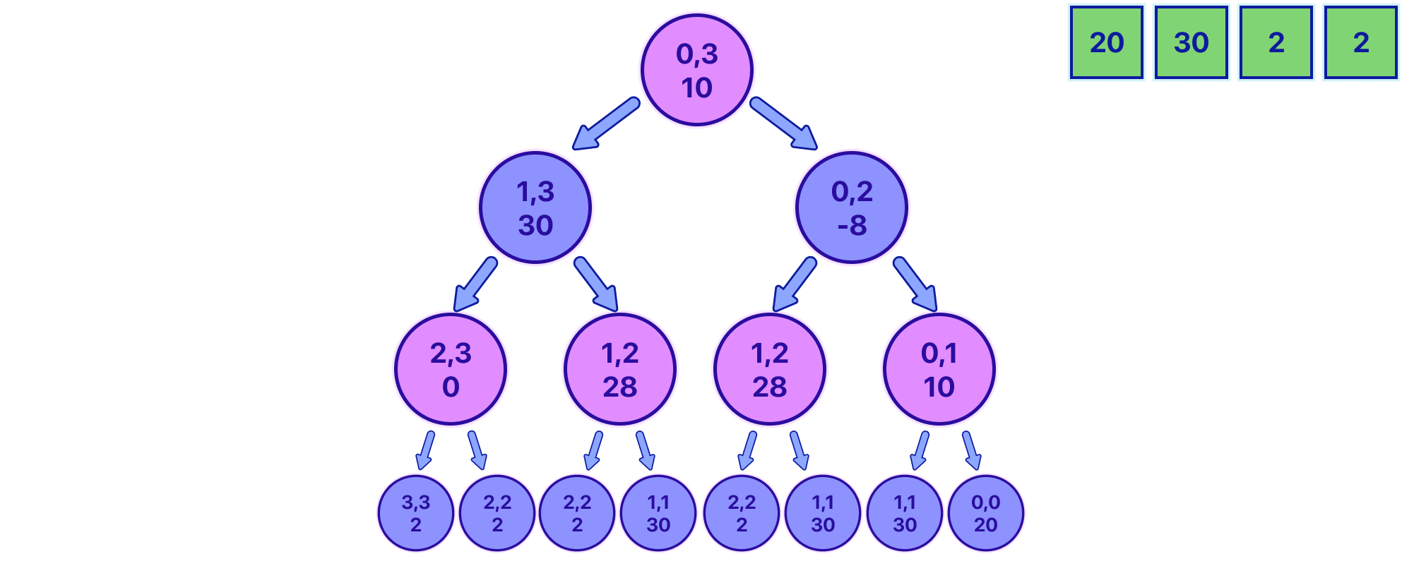
Feel free to take any node and "manually" check if the value is the maximum advantage you are going to have if you start from that node. If we take the root node [0, 3] for example, we can see we end up with an advantage of 10. Let's see why:

• We first pick 2 from the end, leaving the line as 20, 30, 2.

• Our opponent, playing optimally, picks 20, leaving the line as 30, 2.

• We pick 30, leaving the line as 2.

• Lastly, our opponent picks the final 2.

So, playing optimally, we would end up with coins worth 2 + 30 = 32, and the opponent ends up with 20 + 2 = 22.

If we subtract 32 - 22 = 10 we see that the value is indeed correct.

Excellent!, we got the difficult part out of the way, now, knowing the amount by which we beat the opponent (or lose if it's negative) we can calculate our sum using some math.

Let's break down the image above.

1. We start by saying the total amount of coins (T) is made up of your coins (x) and the opponent's coins (y).

2. Next, we say your total coins (x) is made up of your opponent's coins (y) plus the extra coins you managed to snag (d). (d) = the maximum advantage by which you beat the opponent. (or lose if it's negative)

3. Now, we substitute the second equation (x = y + d) into the first (T = x + y). This is like saying the total coins are the same as your opponent's coins, the extra coins you gathered, plus your opponent's coins again. Sounds a bit repetitive, right? But it's crucial for our math to work!

4. Simplifying the above, we find that the total (T) is equal to twice your opponent's coins (2y) plus the coins you snagged extra (d). This is like saying the total coins are the same as two times your opponent's coins plus your extra coins.

5. Rearranging a bit, we subtract your extra coins (d) from the total (T), getting T - d = 2y. This tells us that if we take away your extra coins from the total, we're left with twice the amount of your opponent's coins.

6. Finally, to find your opponent's coins (y), we divide both sides of the equation by 2, which gives us y = (T - d) / 2. This is like saying your opponent's coins are half of the total coins minus your extra coins.

7. We now know the opponent sum, because of this finding yours is simple, it's just x = y + d

And that's it! We've used algebra to solve our problem. It's like a smart way of splitting coins between you and your opponent!

Coded Implementation

As a recap, what we're doing in our solution is exploring every possible move in the game. We do this using a recursive approach, which allows us to create a tree-like map of all potential outcomes. Each node (or possible outcome) tells us the maximum advantage, or benefit, a player can get from a certain range of coins. We define this as:

{LeftIndex, RightIndex, MaximumAdvantage}.

Once we know the maximum advantage possible for the entire range of coins (let's call it 'd'), we can use this in our formula to calculate the final result:

((T-d)/2) + d

Below you can find my fully coded solution in C++

#include <bits/stdc++.h>
using namespace std;
int n, arr[1005]; 

int node(int l, int r){
    if(l == r)return arr[l];
    int left = node(l+1, r);
    int right = node(l, r-1);
    int MaximumAdvantage = max(-left+arr[l], -right+arr[r]);
    return MaximumAdvantage;
}

int main() {
    cin >> n;
    int total = 0;
    for(int i=0; i<n; i++){cin >> arr[i]; total += arr[i];}
    int advantage = node(0,n-1); // [inclusive range]
    int result = ((total - advantage) / 2) + advantage;
    cout << result;
}

As you can see, the code is amazingly simple and short for such a complex appearing problem, there is no need for an actual tree structure implementation with actual nodes and pointers. This is a beautiful example of recursion simplicity.

Time and space complexity

As we saw previously, this solution explores all possible ways the game can unfold:

Notice how for each coin, we have two options - to pick the coin on the left or the right. And for each of these options, we again have two options for the next coin, and so on. Because of this, the number of possibilities we have to check grows exponentially, doubling with each decision, making the time complexity O(2^n).

Given that N = 1000, this code can perform up to 1.07150860718626732094842504906e+301 operations, which of course, it's waaaaaay above our usual 400,000,000 operations limit for most online judges.

This is, in fact, one of the most inefficient time complexities there are. With this solution, the maximum N our solution can process within the limits is approximately N = 30. any value greater than 30 will result in a TLE verdict. 😥

DP Implementation

What if I told you that we can drastically reduce the time it takes to solve this problem? Sounds exciting, right? The solution lies in a clever technique called Dynamic Programming (or DP, for short).

Think about this: while we're exploring all those different ways the game can unfold, we end up checking the same scenarios multiple times. (see image)

That's a lot of wasted effort! Dynamic Programming helps us avoid this by remembering the results of these already-solved scenarios. We call this "memoization".

So, let's use DP to make our program much, much faster. Instead of recalculating results we already have, we can just look them up in our "DP". This way, we save loads of time and avoid repeating work we've already done. We're about to supercharge our program, enabling it to handle more coins and perform its calculations way faster!

Let's see how to implement DP to our coded solution:

#include <bits/stdc++.h>
using namespace std;
int n, arr[1005];
vector<vector<int>> DP(1005, vector<int>(1005, -1));

int node(int l, int r){
    if(l == r)return arr[l];
    if(DP[l][r] != -1)return DP[l][r];
    int left = node(l+1, r);
    int right = node(l, r-1);
    return DP[l][r] = max(-left+arr[l], -right+arr[r]);
}

int main() {
    cin >> n;
    int total = 0;
    for(int i=0; i<n; i++){cin >> arr[i]; total += arr[i];}
    int advantage = node(0,n-1); // [inclusive range]
    int result = ((total - advantage) / 2) + advantage;
    cout << result;
}

Did you spot the new parts? Let's break them down:

1. We've got a DP 'notebook' now. It's like a big grid (or a 2D matrix) where we'll note down results so we can refer to them later. It's sized N * N because that covers all possible combinations of our coin pile indices. And see how it's filled with -1s to start with? That's because 0 could be a valid result, so we need something different to show that we haven't calculated a result yet.

2. We now check our 'notebook' before doing any calculations. If we've already got a result for a particular set of indices, we can just use that instead of doing all the work again. It's like saying, "Hey, we've seen this before! No need to do the same work again."

3. Last but not least, once we've done the calculation for a particular set of indices, we jot it down in our 'notebook' for later. It's like saying, "This could come in handy later. Better note it down."

And there you have it! The same game, the same process, but now supercharged to be much faster. This shows the beauty of Dynamic Programming - the same logic, but a whole lot more efficient!

Time and Space Complexity

Now that we've given our code a dynamic programming boost, you might be curious about how much faster it is and how much more space it needs. Let's look into that:

1. How Fast? (Time Complexity): Before, our code was taking a long time because it was checking every possible coin pick over and over again, which is why the time complexity was O(2^n). But now, thanks to our DP 'notebook', we don't do any calculations more than once. For each possible start and end of the pile (given by the indices), we calculate the result only once and then just look it up whenever needed. So, we've got 'n' possible start points and 'n' possible end points, making it n times n or 'n squared'. Therefore, our new time complexity is O(n^2), which is a whole lot faster!

2. How Much Space? (Space Complexity): We're using a bit more memory in this new code. That's because of our DP 'notebook', the 2D matrix. It's a grid with 'n' rows and 'n' columns, so it has n times n, or 'n squared' spots to store results. So, the space complexity is O(n^2).

In simple terms, we've traded a bit more space to make our program run much faster. And the best part? Now we can solve the game for up to 1,000 coins (where 'n' equals 1,000) without running into any issues since 1,000*1,000 < 400,000,000.

And That's a Wrap! - Farewell

We've reached the end of this deep dive into Dynamic Programming (DP) and how it can supercharge your problem-solving abilities, even in a seemingly complex game like this. And remember, this is not something you'll perfect overnight, it's a skill that takes time and practice to master. So if it doesn't click right away, don't be hard on yourself. This stuff isn't easy, but I hope the walkthrough and explanations provided some clarity and a good foundation to build on.

Remember, we've only just scratched the surface of what DP can do. There's a whole world of interesting problems and applications waiting for you to discover, and while we covered some key concepts and methods here, there's always more to learn.

I hope you've enjoyed this journey as much as I have, and that you've gained some valuable insights and knowledge along the way. I would love to hear your thoughts and any questions you might have. Let me know in the comments!

Thanks for sticking with me till the end, and keep an eye out for more problem-solving adventures! Until next time,