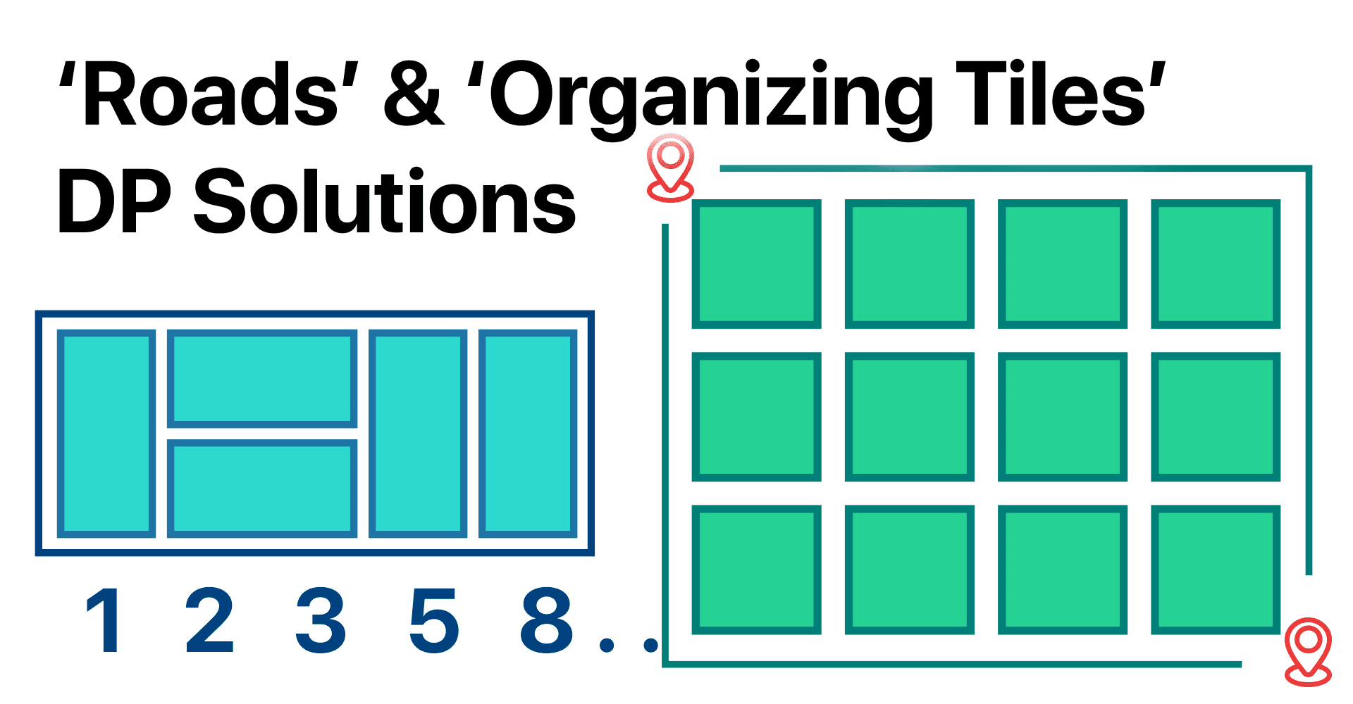
Unveiling Dynamic Programming Solutions for 'Roads' and 'Organizing Tiles' Problems.
👋 Front-End Developer with a flair for competitive programming & robotics. Expert in 3D CAD design, YouTube educator. Innovating from Oaxaca, México.
Introduction
Hello everyone, in this post we will look in detail at the solution to two similar, very classic DP problems: 'Roads' and 'Organizing Tiles', as well as their implementation in C++, altho the solution can be implemented in the language of your choice.
'Organizing Tiles' Problem
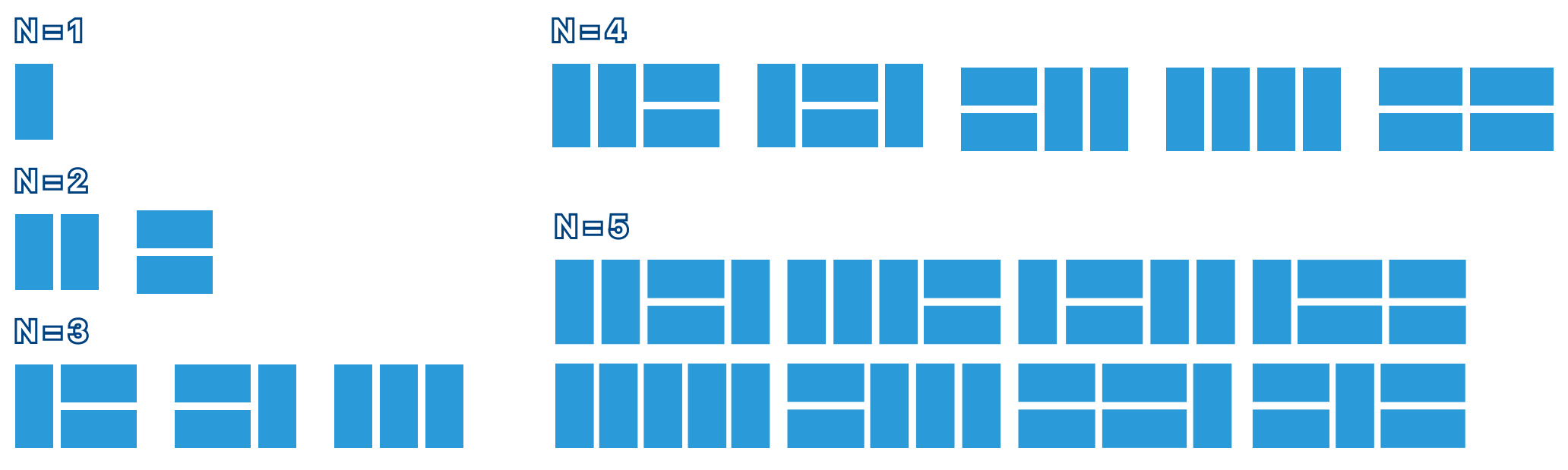
In this problem we need to imagine a rectangular table of size N x 2, this table needs to be completely covered with tiles of size 2 x 1 in such a way that all tiles are completely inside the table and do not overlap, the image below shows all possible valid coverings for a table where N = 4.

you are given T test cases and for each case a single line: N. Output the number of valid ways for covering a grid of size 2 x N.
Inputs
The first line contains T, the following T lines contain a single integer: N.
Output
for each test case output the answer, since the answer can be very large make sure to apply MOD 1,000,000.
Limits
0 <= N <= 1,000,00
1 <= T <= 10,000
'Organizing Tiles' Solution
The first big observation for this problem that we should make is to notice that the height of the table is set to 2 always no matter N, this means that we must only be concerned with the length. Knowing this, a great idea is to manually test and solve the problem as a human for n = 1, n = 2, n = 3, and n = 4. This process can be easily done by drawing all the valid ways we can cover the grid for each N on a notebook.
By doing these drawings, you can clearly see that it's impossible for a valid solution to contain something like this:
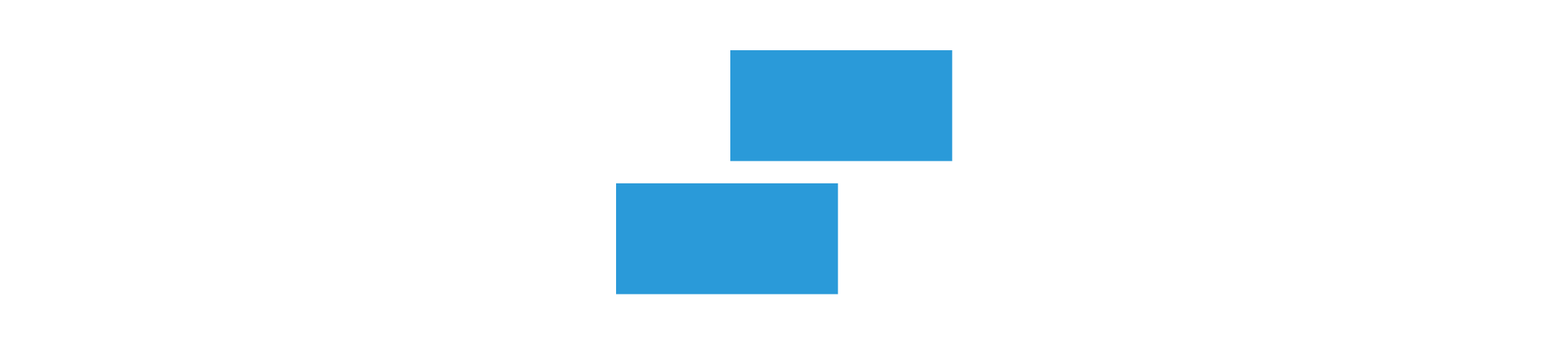
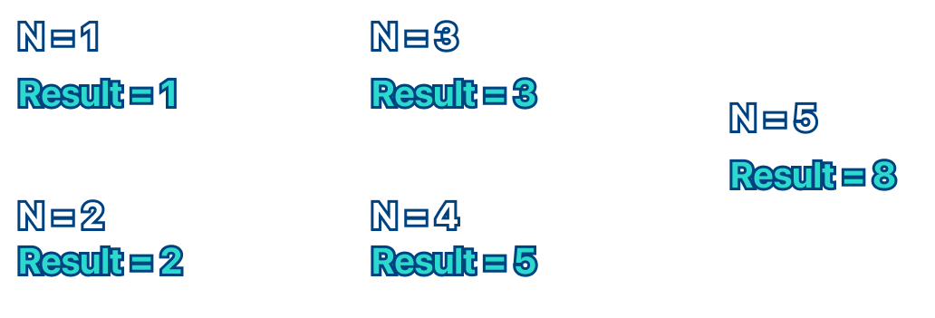
At first sight of the examples, it appears to not have any sort of pattern with the shapes, by observing the coverings for longer we can realize that the shapes themselves don't provide any information in order to predict another N. Because of this we should only pay attention to the number of coverings possible instead of the shapes.
Keeping the idea that the only thing that varies is the length, I started to wonder how can I know the solution for position 5 (1st indexed) without using the drawing method. To answer this question I began by only wondering the amount of ways we can fill that specific index.
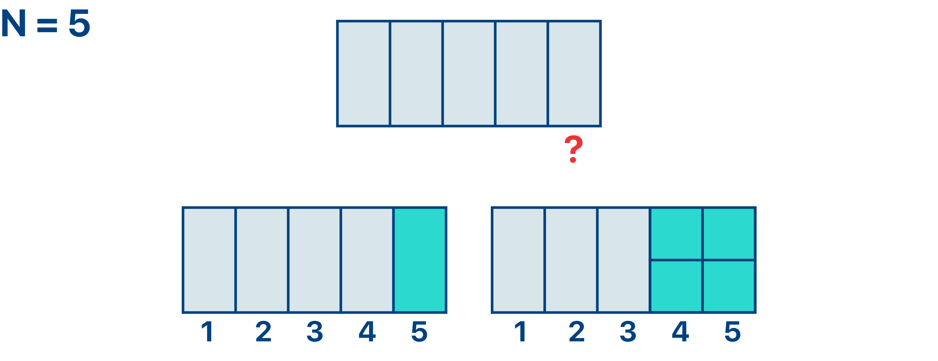
Here is where the interesting solution starts to show. Notice how we have two ways of covering that index. Logically, if we want to know the ways to fill the entire table we should add the possibilities of the remaining space of the first way, with the possibilities of the remaining space of the second. This is looking like a recursive solution, and like most recursive functions we need some base conditions to end it. This case is very easy since we know the answer for N = 0, N = 1, and N = 2;
Recursive Implementation
Below you can find my implementation of the recursive function that solves for N.
typedef long long ll;
ll solve(int n){
    if(n == 0)return 0;
    if(n == 1)return 1;
    if(n == 2)return 2;
    return (solve(n-1) + solve(n-2)) % MOD;
}
Once we code the line solve(n-1) + solve(n-2); it becomes obvious that this code is calculating the Fibonacci sequence. Notice how we are using long long, this is important since the answer can become large, thankfully the problem asks us to apply MOD.

The slight problem with this implementation is that for every N query, the recursion will be redone until one of the base conditions is fulfilled, this is very inefficient. however, we can use DP (Dynamic Programming) to compute the solution for N so that if it at some moment N gets repeated we can simply return the pre-computed answer.
typedef long long ll;
ll DP[1e6 + 5], MOD = 1e6;
ll solve(int n){
    if(n == 0)return 0;
    if(n == 1)return 1;
    if(n == 2)return 2;
    if(DP[n]) return DP[n];
    return DP[n] = (solve(n-1) + solve(n-2))%MOD;
}
in the code cell above you can see the DP container added, now in our solve function, if a solution for N is already computed in the DP we return the value, else, we compute the solution and save it to the DP.
return DP[n] = solve(n-1) + solve(n-2);
this is a fancy way of assigning the answer to the DP and returning the value in a single line.
Iterative Solution
since the solution to this problem is simply to calculate the Fibonacci sequence, there is no need to use recursion, and you can do something iterative like this:
typedef long long ll;
vector<ll>fib = {0,1,2};
ll MOD = 1e6;
int main(){
    ll n; cin >> n;
    for(ll i = 2; i <= 1e6 + 5; i++){
        fib.push_back((fib[i]+fib[i-1])%MOD);
    }
    cout << fib[n]%MOD;
    return 0;
}
Time and Space Complexity
Recursive Solution
Time Complexity: The time complexity of this algorithm is O(n), where
nis the input to the function. This is because each function call to solve for a particular value ofnis made only once due to memoization. Oncesolve(n)is calculated, its value is stored in the DP array. Therefore, the total number of operations is linear with respect to the input size, leading to a time complexity of O(n).Space Complexity: The space complexity of this algorithm is also O(n), where
nis the input to the function. This is because an array of sizen(specifically n + 5, but we ignore constants in Big O notation) is created to store the results of the function for each possible value of n from 0 to n. Thus, the amount of memory used scales linearly with the size of the input, leading to a space complexity of O(n).
Iterative Solution
Time Complexity: The time complexity of this code is O(n), where
nis the maximum number for which you want to compute the Fibonacci number. This is because there is a loop that iteratesntimes, and within each iteration, you perform a constant amount of work: retrieving two elements from the vector, adding them, taking the modulus, and appending the result to the vector. All of these operations are assumed to take constant time. Thus, the total amount of work done is proportional ton, leading to a time complexity of O(n).Space Complexity: The space complexity of the code is also O(n). This is due to the
fibvector, which storesnelements. Since the amount of space used by the vector scales linearly withn, the space complexity is O(n).
'Roads' Problem
Imagine that there is a city represented by a rectangular grid of size H * W, where H is the height of the grid and W is the width. (See picture)
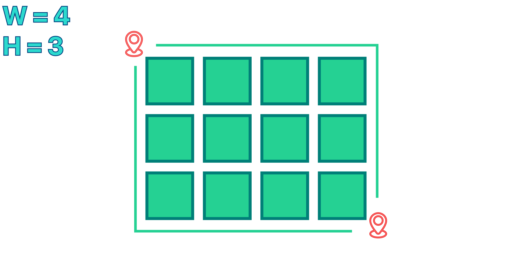
Jhon lives in the left top corner of block {0, 0}. you need to help him figure out the number of ways he can reach his parent's house which is located in the bottom right corner of the grid, by only moving to either right or down.
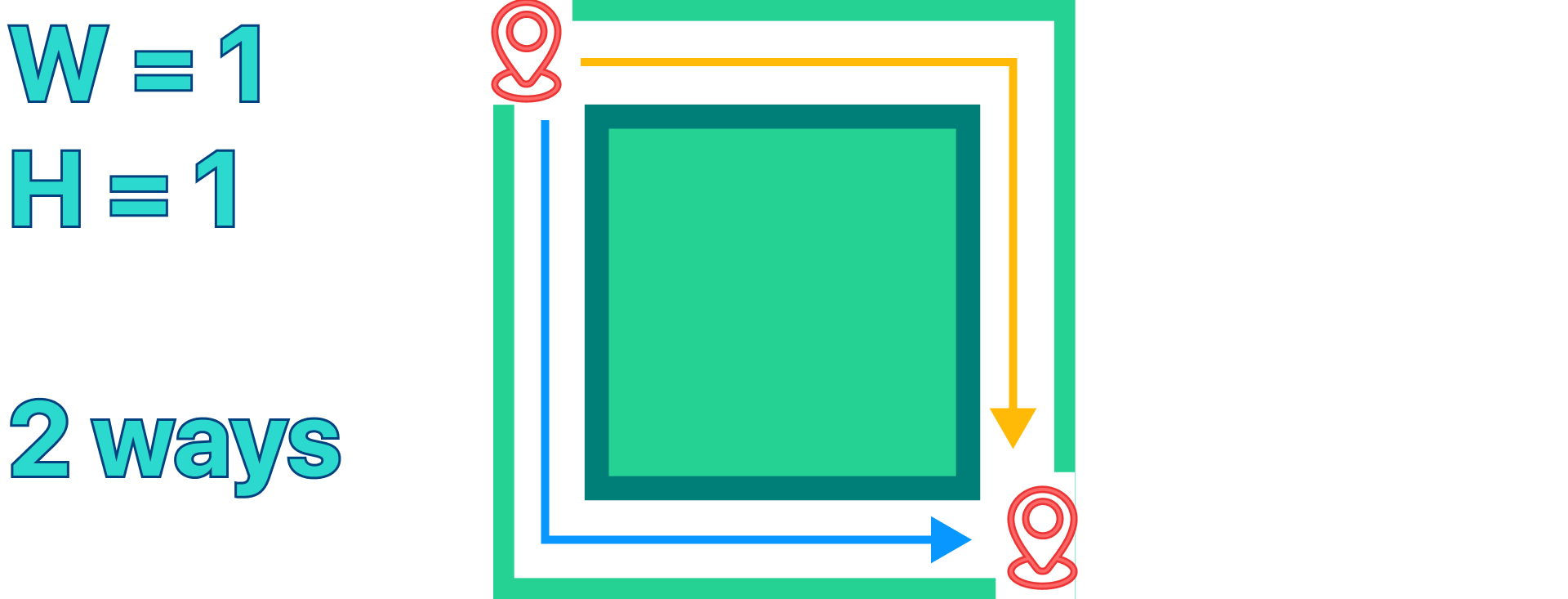
Note: Jhon moves through the "roads" which are represented by the edge of the block, for better understanding look at the picture below in which W = 1 and H = 1;
Inputs
The first and only line contains integers W and H, representing the height of the grid,
Output
Your code must output a single integer, the number of distinct ways for Jhon to reach his parent's house.
Limits
- 1 <= W, H <= 30
'Roads' Solution
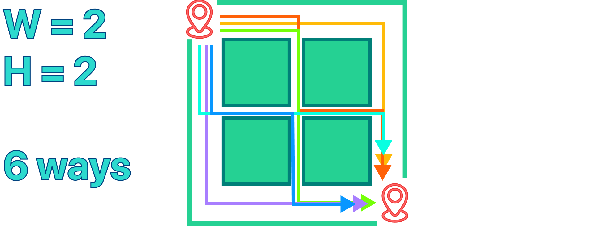
As we usually do when solving a problem, it's a good idea to solve the problem as a human for a couple of examples with the help of a notebook and make drawings of all paths to better understand the relationship between input and output.
Recursive Solution
When doing this manual process we can figure out a first brute-force approach of trying all possible paths. This can be done with a recursive function solve(int x, int y) that tries the two different paths solve(int x + 1, y) + solve(int x, int y + 1);
Let's see how such a solution can be implemented.
#include <bits/stdc++.h>
using namespace std;
typedef long long ll;
int w, h;

ll solve(int x, int y){
    if(x > w || y > h)return 0;
    if(x == w && y == h)return 1;
    return solve(x+1, y) + solve(x, y+1);
}


int main() {
    cin >> w >> h;
    cout << solve(0,0);
    return 0;
}
as you can see the solve solution only uses three lines of code, one condition to see if we have reached the bottom right corner (therefore a path exists), and we also check if it's inside the bounds of the map.
Unfortunately, because this code tries all different paths possible, it means that the Time Complexity In the worst case is O(2^(w+h)) because the function solve will be called for every possible pair (x, y) where x is in the range [0, w] and y is in the range [0, h]. However, due to the nature of the recursive calls (moving right or down), many of these calls will be made multiple times for the same pair of coordinates, leading to a large number of redundant operations. This, of course, is exponential. Given that W and H can be up to 30 this means that approximately 2^60 operations are going to be computed, which of course exceed the 400,000,000 operations that are normally the limit for most online judges. This solution is going to receive a TLE (Time Limit Exceded) verdict. However, because there are repeated solve(x, y) calls, it means that we can apply DP.
#include <bits/stdc++.h>
using namespace std;
typedef long long ll;
ll w, h, DP[31][31];

ll solve(int x, int y){
    if(x > w || y > h)return 0;
    if(x == w && y == h)return 1;
    if(DP[x][y])return DP[x][y];
    return DP[x][y] = solve(x+1, y) + solve(x, y+1);
}

int main() {
    cin >> w >> h;
    cout << solve(0,0);
    return 0;
}
by doing this very slight code addition we are Reducing Redundant Calculations, In the previous version of the code, the same calculations were performed many times due to overlapping sub-problems. For example, both solve(1, 2) and solve(2, 1) would end up recursively calculating the result for solve(2, 2), among other overlapping calculations. This redundancy leads to an exponential time complexity, which is highly inefficient. However, with DP, the result of each unique call to solve(x, y) is stored in the DP[x][y] array after it's calculated for the first time. Then, if solve(x, y) is called again, the function will first check if DP[x][y] is non-zero, and if so, it will immediately return this stored result instead of re-calculating it. By applying this technic we managed to reduce the 2^60 operation to just 60 🤯.
Iterative Solution
Altho the previous solution is already enough to receive an AC verdict (accepted) it is not the only correct implementation to get it. I made this very cool observation when printing out the DP from the previous solution:
35 15 5 1
20 10 4 1
10 6 3 1
4 3 2 1
1 1 1 0
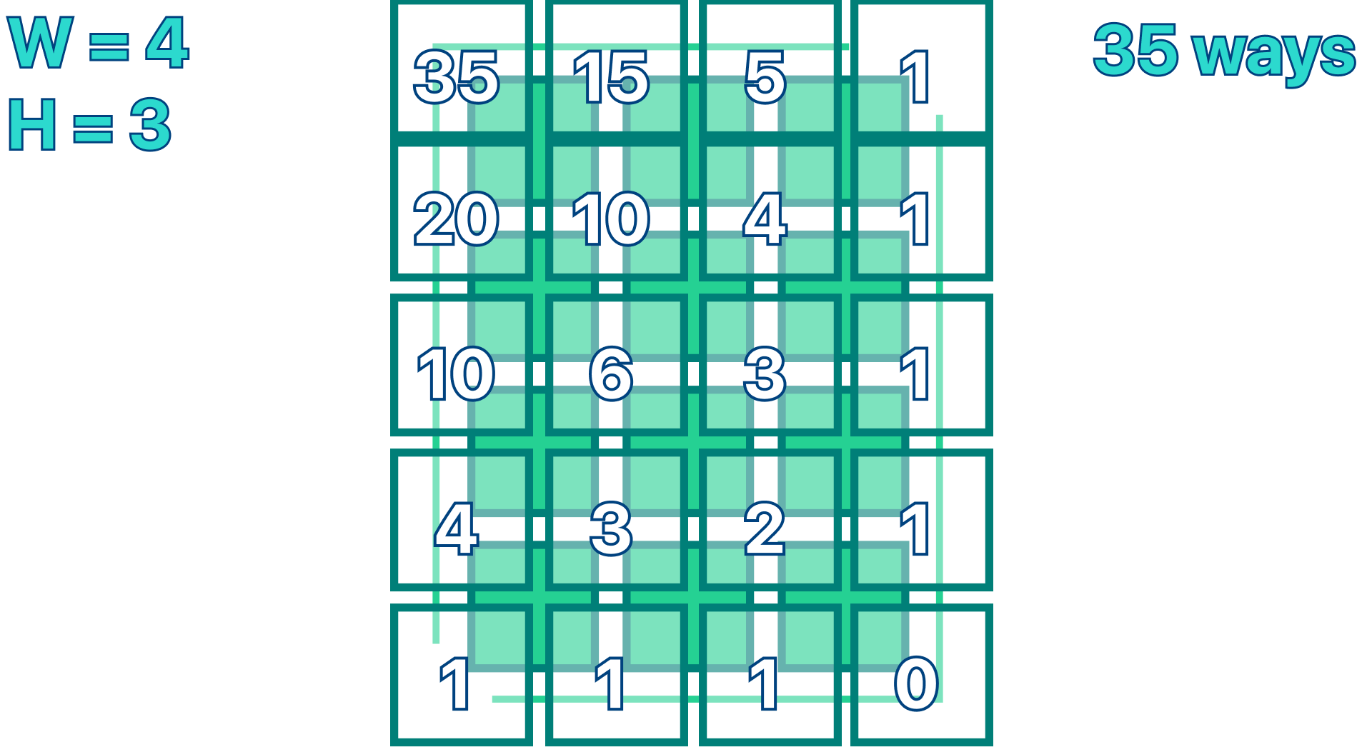
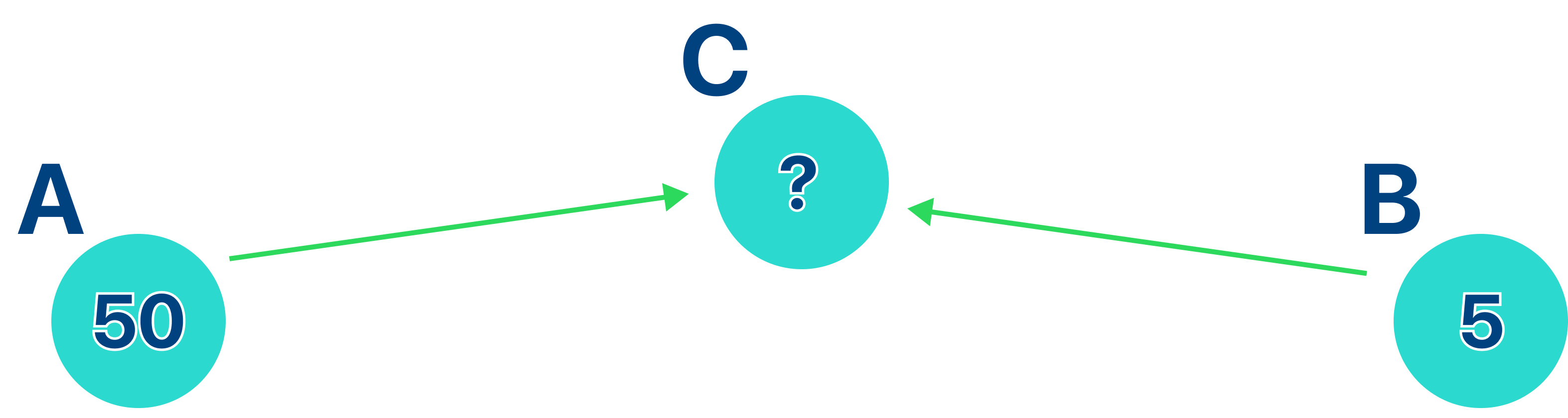
First of all, notice how the orientation of the table does not matter. Then, if we look closely the value clearly represents the number of ways for reaching a certain point if we start from the end which happens to always be the sum of the ways we can reach the cell below, with the ways we can reach the cell in the right. This makes a lot of sense, since if we can reach point A in 20 ways, and point B in 5, and we want to know the number of ways we can reach point C, it's trivial that it's the sum of 20 + 5.
By knowing this, we can initialize a DP matrix in which all the values in the first row and the first column are set to 1, this is going to be our base case since as we can confirm in our image there is always 1 way only to reach any of the points of the first row and the first column. (see image)
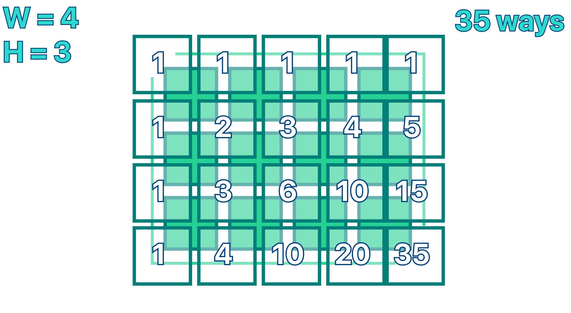
Then we can fill the rest of the table by iterating square by square and making the value of the point equal to the ways we can reach the point above, with the ways we can reach the point on the left. Lastly, we can just access the point {H, W}.
Here is my code implementation:
#include<iostream>
using namespace std;
typedef long long ll;

int main(){
    ll H, W; cin >> H >> W;
    ll DP[H+1][W+1];
    for(int i=0; i<=W; i++)DP[0][i] = (ll)1; // filling the first row
    for(int i=0; i<=H; i++)DP[i][0] = (ll)1; // filling the first column
    for(int i=1; i<=H; i++){
        for(int j=1; j<=W; j++){
            DP[i][j] = DP[i-1][j] + DP[i][j-1]; // filling DP
        }
    }
    cout << DP[H][W];
    return 0;
}
Time and Space Complexity
Recursive Solution
Time Complexity:
The primary operations in this algorithm are done in the
solvefunction, where it calculates the number of paths from (0,0) to (w,h).The number of distinct problems to be solved is
w*h, wherewis the width andhis the height of the 2D grid. This is because we need to compute the number of paths for each cell from (0,0).The time complexity of each problem is O(1). This is because the function
solveeither returns the stored result in DP[x][y] (if it has been computed before), or it computes the result as the sum ofsolve(x+1, y)andsolve(x, y+1). Both of these are O(1) operations because they are simple mathematical operations or array accesses.
Therefore, the overall time complexity of this algorithm is O(w*h).
Space Complexity:
The space complexity is also O(wh) because of the 2D DP array used to store the intermediate results. Each cell in the grid has a corresponding cell in the DP array, thus leading to wh cells in the DP array.
The 2D array
DPis of size [31][31], but the actual space used will be w*h wherewandhare the width and height of the 2D grid. This is the space needed to store the number of paths for each cell.
Iterative Solution
Time Complexity:
The time complexity of this program is determined by the double for-loop that iterates over all the cells in the grid to calculate and fill in the DP array.
The outer loop runs H+1 times (from 0 to H) and for each iteration, the inner loop runs W+1 times (from 0 to W).
Inside the inner loop, you're performing a constant amount of work (accessing elements in the DP array and adding them together).
Given this, the time complexity is O(H*W).
Space Complexity:
The space complexity of this program is determined by the size of the DP array.
The DP array is of size (H+1)x(W+1). You need to store a long long integer for each cell in the grid, which gives a space complexity of O(H*W).
Besides the DP array, the rest of the variables occupy constant space that does not grow with the size of the input.
Therefore, the overall space complexity is O(H*W).
Conclusion - Farewell
We've explored two dynamic programming (DP) problems in-depth - 'Organizing Tiles' and 'Roads'. Both were tackled with recursive and iterative solutions, helping us appreciate the versatility of DP. By analyzing time and space complexity, we've learned about performance trade-offs in different scenarios.
Dynamic Programming is a powerful technique, breaking down problems into manageable sub-problems. It's essential in competitive programming and beyond. Remember, mastering DP needs practice and intuitive understanding. Identify overlapping subproblems, understand them, and choose between recursion or iteration as per the constraints.
Keep practicing and learning. Every problem solved takes you closer to mastery. The learning journey is as rewarding as the destination itself, enriching you with invaluable skills.
Thank you for joining this DP journey. I hope it's been insightful and encourages you to solve more DP challenges. Until next time, happy coding and stay curious!