Mastering The "k-Tree" Problem with Dynamic Programming
👋 Front-End Developer with a flair for competitive programming & robotics. Expert in 3D CAD design, YouTube educator. Innovating from Oaxaca, México.
The K-Tree Problem
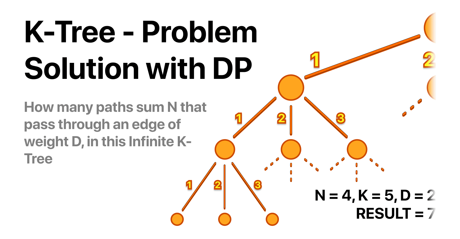
A k-Tree is a unique tree structure where each node has exactly k children nodes, extending infinitely. The tree is weighted, such that each of the k edges stemming from a node carries a weight value ranging from 1 to k. In the illustration below, we have an example of a k-tree where k equals 3.
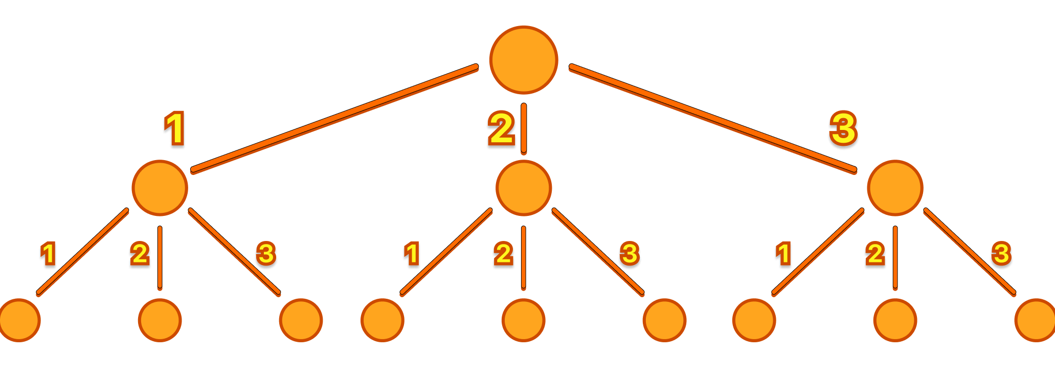
Please note that in this particular image, the tree is depicted to a depth of 3. However, remember that a k-tree is infinite, and this pattern of branching continues endlessly from each child node.
Now, let's consider the following problem:
Given three parameters K, N, and D, write a program that answers the following question:
'How many paths are there starting from the root node, such that the total sum of the edge weights in a path equals N, and the path includes at least one edge of weight D or more?'
Inputs
A single line containing three integers: N, K, and D.
Constraints:
- 1 <= N, K <= 100
- 1 <= D <= K
Outputs
A single integer: the answer to the problem. Given that the answer can be quite large, ensure to output your answer modulo 10^9 + 7.
Examples
Example 1:
Input: 3 3 2
Output: 3

Example 2:
Input: 3 3 3
Output: 1

Example 3:
Input: 4 5 2
Output: 7
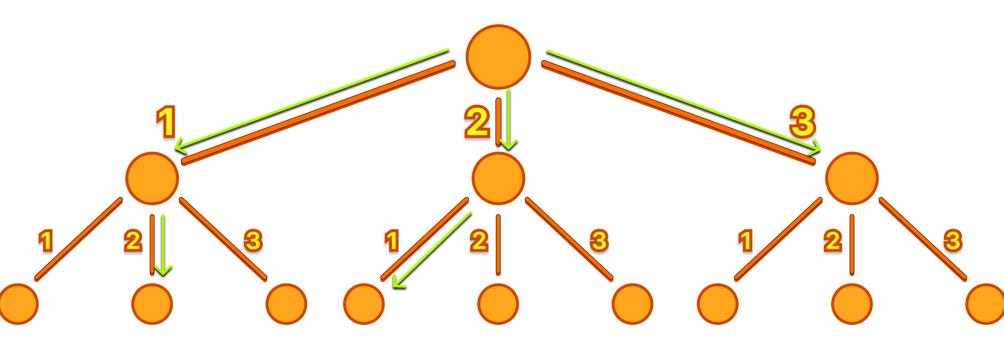
Here is an image for the first example:
Problem-Solving as a Human
When tackling a problem, it's often best to start by examining an example and trying to solve it logically, as a human would. In this case, it's helpful to sketch out a tree for the first example to understand the relationship between the input and output. The first and most apparent solution was to model the tree structure and attempt to traverse all possible paths.
Pausing to Evaluate the Approach
Before diving into implementing this approach, let's pause and consider potential challenges. The first thing I noticed is that the tree's "nodes" are irrelevant - they carry no intrinsic value. We are only interested in the edges, and the order in which we traverse the tree doesn't matter. Moreover, the tree is infinite, which could lead to complications during implementation.
With these insights, I decided to reassess the situation, returning to the drawing board. But this time, instead of focusing on the tree, I would only consider the edge values.
Solving the Problem Without the Tree
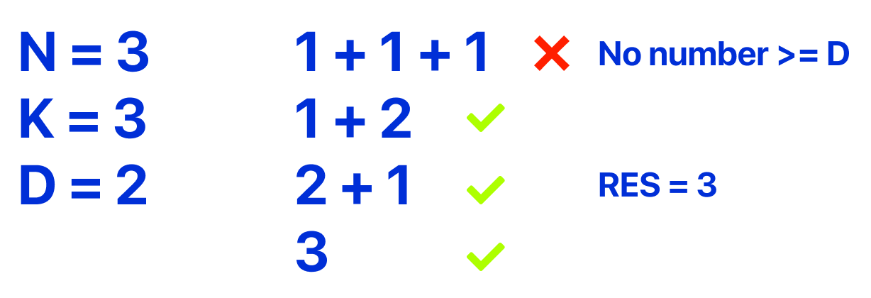
For the first example, I wrote down the variable values. This reminded me of three key points:
The sum of the path should be exactly N
All Edges used must be less or equal to K
A path is valid only if there is an edge with a weight greater than or equal to D.
Taking these points into account, we can rephrase the problem as:
"How many ways can you form a sum equal to N using numbers less than or equal to K, with at least one number being greater than or equal to D?"
This greatly simplifies the problem since we have effectively removed the "tree" aspect from it. Now, we can solve the problem using only numbers and we can still maintain the same basic approach of testing all possible number combinations.
Solution Pseudo Code
For problems involving combinations, a recursive function often comes in handy. However, it's crucial to define base cases and divide the problem into manageable components. In this scenario, we'll start with:
"How many ways can you form a sum equal to N using numbers less than or equal to K, with at least one number being greater than or equal to D?"
Base cases for the first part:
Since the Tree is infinite, we need a condition to stop the current path when the sum exceeds N. This is important as further exploration of this path won't yield a valid solution (given that there are no negative edges).
We need to acknowledge when we've successfully formed a sum equal to N. This involves incrementing our answer count and halting the current path exploration.
With these two considerations, let's lay out the following pseudo code:
N = 3, K = 3
RESULT = 0
function solve(sum):
    if sum > N: return
    if sum == N: {RESULT += 1; return}
    for each number from 1 to k:
        solve(sum + number)
now let's consider the second part of the problem:
"How many ways can you form a sum equal to N using numbers less than or equal to K, with at least one number being greater than or equal to D?"
Base cases for the second part:
We're interested in whether there's at least one number greater than or equal to D. To capture this, we add a boolean parameter to our function,
valid, which becomes true if a number meets this condition.Additionally, we need to modify the base case that increments the result. Now, we should only increment if
validequals true.
Combining both problem parts, we can arrive at our final pseudo code:
N = 3, K = 3, D = 2
RESULT = 0
function solve(sum, valid):
    if sum > N: return
    if sum == N and valid: {RESULT += 1; return}
    for each number from 1 to k:
        solve(sum + number, number >= D or already valid)

solve(0, false)
print(RESULT)
Code Implementation
I highly recommend trying to implement the solution in your preferred programming language. Below is my implementation in C++:
#include <bits/stdc++.h>
using namespace std;
int N, K, D, RES = 0;

void solve(int sum, bool valid){
    if(sum > N)return;
    if(sum == N && valid){RES++; return;}
    for(int i=1; i<=K; i++)solve(sum + i, i >= D || valid);
}

int main() {
    cin >> N >> K >> D;
    solve(0, false);
    cout << RES;
    return 0;
}
Time and Space complexity
The worst-case time complexity is exponential, O(K^N), as the function solve can potentially make K recursive calls at each depth level, with the maximum depth level being N. However, the actual time complexity will likely be significantly less than O(K^N) due to the early return condition (if(sum > N)return;) which prunes many branches of the recursion tree where the sum has already exceeded N.
The space complexity is O(N), which represents the maximum depth of the recursive call stack. Each recursive call adds a new level to the stack.
However, keep in mind that the time complexity for this solution is not desirable given that N and K can be up to 100. This could result in up to 1.e+200 operations, which is far beyond what can be executed without encountering a Time Limit Exceeded (TLE) verdict.
Optimizing Our Solution
Whenever I create a recursive solution that tests for all possibilities and it needs optimization, the first thing I check is the possibility of repeated function calls, or what I call "repeated states".
What is the state of our solution?
In this specific solution, the state is represented by the parameters of the function {sum, valid}. Both values are critical to defining the state.
Identifying repeated states
An easy method to identify repeated states is to add a print statement in our function like this:
void solve(int sum, bool valid){
    cout << "{ " << sum << " , " << valid << " }\n";
By running the code with input: 4, 5, 2, it becomes evident that state { 6, 1 } is repeated eight times.
Implementing Dynamic Programming (DP)
If repeated states exist, it indicates that Dynamic Programming (DP) can be applied to optimize the code. DP involves computing the solution for a state, storing it, and reusing it whenever the state is encountered again. This approach saves significant computation time.
Here's the C++ implementation utilizing DP:
#include <bits/stdc++.h>
using namespace std;
int N, K, D;

vector<vector<int>> DP(105,vector<int>(2, -1));

int solve(int sum, bool valid){
    if(sum > N)return 0;
    if(sum == N && valid)return 1;
    if(DP[sum][valid] != -1) return DP[sum][valid];
    int resultForThisState = 0;
    for(int i=1; i<=K; i++){
        resultForThisState += solve(sum + i, i >= D || valid);
    }
    return DP[sum][valid] = resultForThisState;
}

int main() {
    cin >> N >> K >> D;
    cout << solve(0, false);
    return 0;
}
Breaking Down the DP Implementation
This code is similar to the original recursive solution with the addition of a DP approach. Let's look at the new elements in detail.
vector<vector<int>> DP(105,vector<int>(2, -1)); This line of code initializes our DP storage. It's a 2D matrix of size 105x2. We use 105 as the size because, although N can only reach 100, it's a good practice to leave a little margin for error. The second dimension is 2, as valid is a boolean variable and can only have two values (true or false).
Note: The entire matrix is initialized with -1. This is critical because 0 can be a valid computed answer.
if(DP[sum][valid] != -1) return DP[sum][valid]; This line checks if there's a precomputed result for this state. If there is, it returns that value, saving us from unnecessary computation.
if none of the base case conditions are met, we store the result for the current state, which is the sum of all of its children's results.
return DP[sum][valid] = resultForThisState; This line stores the result of the current state in the DP table and returns that value. It's a concise way of accomplishing two tasks at once.
Time and Space Complexity
This solution using Dynamic Programming has considerably improved the time and space complexity compared to the previous recursive solution without memoization.
Time complexity: The time complexity of the function is O(NK), since the function solve is called for all sums from 0 to N (N+1 states), and for each sum, there are K possibilities to consider. But due to memoization, each state {sum, valid} is computed only once, giving us a time complexity of O(NK).
Space complexity: The space complexity of the program is O(N) due to the DP array, which has a size of 105x2. The recursion stack in this case doesn't contribute significantly to the space complexity because once a state is computed, it is stored and doesn't need to be computed again. The 2D DP array size is constant (105x2) and does not depend on the inputs N, K, or D. Therefore, the space complexity is O(1). However, considering that the size of the DP array is proportional to N, it could also be considered as O(N) in terms of input size.
So, we can say that the time complexity is O(N*K) and the space complexity is O(N) (or O(1) if considering the fixed size of the DP array).
This is incredibly efficient because N and K can be up to 100, this means that at most, this code runs 10,000 operations. 😎🥳
Full Code + Small Corrections
Two small details we left out in our coded solution were: "Given that the answer can be quite large, ensure to output your answer modulo 10^9 + 7."
However, this can be added very simply by using the C++ long long data type for large numbers and adding the Modulo operation every time the solve() function gets used.
#include <bits/stdc++.h>
using namespace std;
typedef long long ll;

int N, K, D;
ll MOD = 1e9 + 7

vector<vector<ll>> DP(105,vector<ll>(2, -1));

ll solve(ll sum, bool valid){
    if(sum > N)return 0;
    if(sum == N && valid)return 1;
    if(DP[sum][valid] != -1) return DP[sum][valid];
    ll resultForThisState = 0;
    for(ll i=1; i<=K; i++){
        resultForThisState += solve(sum + i, i >= D || valid) % MOD;
    }
    return DP[sum][valid] = resultForThisState % MOD;
}

int main() {
    cin >> N >> K >> D;
    cout << solve(0, false) % MOD;
    return 0;
}
Conclusion + Farewell
In conclusion, solving a competitive programming problem requires an understanding of the problem statement, the ability to break down the problem, and knowing the right approach to use. The k-Tree problem provided a clear illustration of these steps, taking us from an initial analysis and solution that wasn't efficient, to a significantly more efficient solution using Dynamic Programming.
Don't be disheartened if you don't immediately see how to solve a problem. The beauty of competitive programming is in the journey and the learning process. With practice and a determination to understand the concepts, you will continually improve. Always remember to keep refining your skills, keep learning, and most importantly, enjoy the journey!
We hope you found this article useful and educational. Stay tuned for more competitive programming problem breakdowns and insights. Happy coding!


